Fertility from a Bayesian perspective – worth trying?

This guest post by Beata Osiewalska discusses and describes her research on Bayesian approaches in fertility analysis.

Is it possible to see the probability distribution over the number of children for a person with some particular demographic or socio-economic background? Have you ever wondered what this distribution would look like in your case? In this article I will present the methodological framework to achieve this goal, and the nut and bolts behind it.

Many researchers already appreciate the usefulness of the Bayesian approach for migration and population projections or forecasting (Land 1986, Pflaumer 1998, Daponte et al. 1997, Bijak 2011, Raftery et al. 2012, Bryant and Graham 2013). However, demographers in other areas, e.g. fertility, are still not familiarized with Bayesian methodology, and the opportunities it gives are not entirely exploited.

You may be asking: what are these opportunities? In response, I can also pose a question: what about our previous research and all the knowledge that we get from them? Do we really have to forget about everything that we already know each time we start a new analysis? Surely not! In the Bayesian approach we can naturally and coherently include our initial knowledge into the model, as well as update the model as soon as new facts emerge.

The next is uncertainty issue, the importance of which we tend to ignore in our analyses, especially when the inference refers to non-linear functions of model parameters, for which we usually obtain wide confidence intervals. In Bayesian analyses, non-linearity does not require asymptotic properties anymore and uncertainty is still as precise as possible.

Let me mention a few more – the small sample size problem, a huge limitation in the classical approach,  is not an issue anymore in Bayesian modeling with properly chosen prior distributions; and finally, the computational advantage of Bayesian approach which becomes evident when it is numerically complex to find the global extremum of the likelihood function (because the prior distribution acts as a regularizer) or the detailed posterior knowledge.

How  can a proper fertility model be found?

Going back to the area of fertility – the measured outcome (the number of children) has a specific nature –zero that stands for childlessness and positive numbers (1,2,…) for parenthood. Behaviour could be driven by different factors in each state (childlessness and parenthood). Therefore, we are obliged to consider a model that allows treating childlessness as a qualitatively different state than having children. The Zero-Inflated Poisson (ZIP) seems to be a perfect choice – it consists of two states, zero and count, and gives the opportunity for us to set up different determinants in modeling childlessness (zero) than in modeling parenthood (counts). The formula is a combination of  logistic and standard Poisson regressions:

Zero-Inflated Poisson Formula

Modeling the transmission of fertility pattern

To show an example of using Bayesian ZIP model in the area of fertility, let’s consider the transmission of fertility pattern from a mother to her daughter. Previous results suggested that a daughter’s number of children is positively correlated with the mother’s fertility pattern (Pearson et al. 1899, Murphy 1999, Booth and Kee 2009, Kolk 2011, 2013), and that the effect is stronger in developed countries. Using contemporary data (1^st wave GGS dataset for Austria) we will check the influence of number of siblings and mother’s age at the daughter’s birth (as a proxy of mother’s age at childbearing) on the daughter’s number of children.

Including initial knowledge

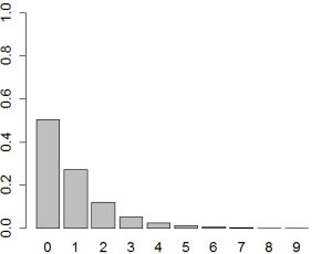
First, let us define prior distribution as a reflection of initial knowledge or our beliefs. Intuitively, a good prior should fulfill two conditions: enable all reasonable values and remain coherent with common knowledge. In case of a hypothetical woman, most would agree that the prior distribution should set higher probabilities for smaller numbers of children (from zero to 3), and at the same time very low probabilities (even equal to zero) for numbers of children greater than or equal to 10 (see Figure 1).

Figure 1. The prior distribution of number of children for a chosen woman

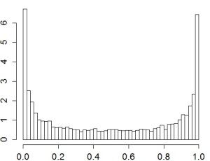
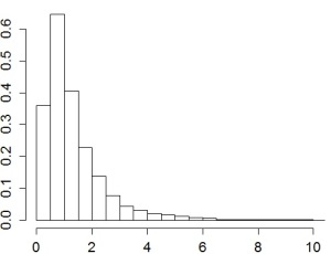
Regarding the probability of childlessness, we would rather like to have values close to zero or close to 1, because we would want to be sure whether someone will be childless or not (see Figure 2a). In turn, the average number of children is a priori expected to take again rather smaller values (as reflected on Figure 2b).

Figure 2a. The probability distribution for a chosen woman

Figure 2b. The lambda distribution for a chosen woman

The comprehensiveness of posterior results

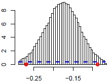
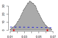
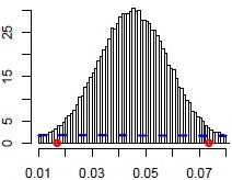
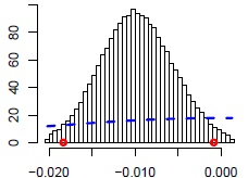
Let us focus now on the marginal posterior distributions of all considered parameters, which are useful to check the shape of the distributions (Unimodal? Symmetric? And most important: does the posterior indicate we have learned something additional from the data, so whether the posterior is different than the prior?) and visually determine the impact of the parameter on the modeled variable (see Figures 3a-3d with marginal a posteriori distributions of chosen parameters).

Figure 3a. Zero model: number of siblings

Figure 3b. Zero model: mother’s age at respondent’s birth

Figure 3c. Count model: number of siblings

Figure 3d. Count model: mother’s age at respondent’s birth

Based on the posterior distributions (Figures 3a-3d) we could say that fertility pattern developed in the origin-family home showed an important effect on a woman’s procreative behavior. The more siblings a woman has, the lower the posterior probability of being childless (ZERO model) and the higher the chance of having bigger family (COUNT model). Subsequently, the older the mother was at the respondent’s birth, the higher risk of being childless and the lower the posterior probability of having many children by a daughter.

Taking advantage of detailed posterior knowledge

Additionally, let’s also consider two profiles (type A and B), defined in order to demonstrate the procreative behaviors of women with different family backgrounds, and let’s build a posterior distribution of expected number of children in both cases (see Figure 4). The differences are visible and important and uncertainty is still relatively low (regardless of the nonlinearity of the considered measure). When a woman grew up with many siblings, it is much more probable that she will follow the same pattern in her own family. A woman with 4 siblings would probably have 2 children (the a posteriori expected value is 2.014), while among women with no siblings, one in three would have only one child (the a posteriori expected value is 1.699). Additionally, we can see that when a mother gave birth to a daughter at an older age, that daughter will probably have fewer children. The a posteriori expected number of children for a woman, whose mother was 18 at her birth, is 1.783, and 1.316 for those whose mother was 45.

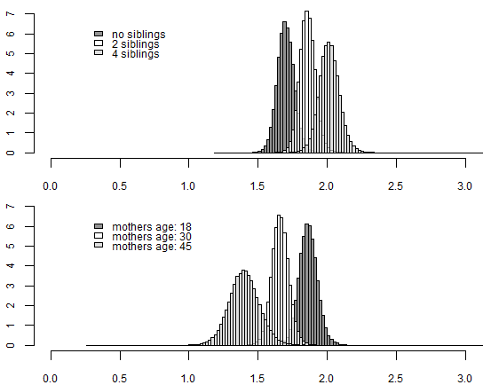
Figure 4. The posterior distributions of expected number of children for type A (top) and B (bottom)

It should be noted that in order to analyze the fertility by females’ profiles, the Bayesian approach was crucial. Inference about these distributions would be impossible within the classical approach – we would not be able to obtain full knowledge about the distributions of nonlinear functions of parameters, such as the probability of childlessness or expected number of children.

The Zero-Inflated Poisson model and Bayesian inference seems to form a useful framework for analyzing fertility, especially when the particular research interest is in the total number of children (actual or intended). The ZIP model gives a different qualitative dimension (value) to childlessness and parenthood and simultaneously keep these two states under the one fertility model – so possible dependencies between those states (one state is connected to the other by the probability of childlessness/parenthood) are allowed. The Bayesian approach, in turn, provides us with precisely estimated results and helps to deal with many other computational and data issues.

Beata Osiewalska is a Research and Teaching Assistant at the Demography Department of the Cracow University of Economics, Poland. Her PhD topic (in progress) is about Bayesian analysis of the relation between fertility and couples’ socioeconomic status. In case of any ideas for improvement, contact beata.osiewalska@uek.krakow.pl. If you are interested in methodological details or want to know more about the transmission of fertility pattern see the full paper here.

Tags: Austria, Bayesian methodology, GGS