Forecasting the outcome of the World Cup

The World Cup begins this week, in the face of controversy over corruption and venality in FIFA and continuing protests in the host nation Brazil against the incredible cost of the tournament and the harsh crackdowns on favela residents. Apart from the obvious moral and political debates, there are interesting demographic angles that could be taken on this topic: the World Population Prospects show that Brazil has a young population, with more than half the population under 30, and such a demographic bulge has been suggested by some to be a potential cause of unrest. Similarly inequality is rife in the Brazil, and is perhaps the root of much of the discontent: demographic approaches to this topic abound.

Who will win in Brazil?

Leaving these issues to those better able to discuss them, however, I’d like to focus on something much less serious. The statistical tools used by demographers and social scientists were often initially developed with the purpose of predicting games of chance. As demographers, forecasting and prediction is a large part of our day job, and so it seemed appropriate to use this post to attempt to predict the outcome of the World Cup.

I adopt a simple Bayesian hierarchical model for the prediction of the results of football matches developed by Baio and Blangiardo, and fit this to past international results. The estimated model parameters are then used to simulate the eventual winners of the tournament.

The model is based upon the assumptions that the number of goals scored by a team follows a Poisson distribution, implying that goals occur at a constant rate over the match, and that the number of goals by one team is independent of the number scored by their opposition (conditional on the model hyper-parameters). The parameter controlling the Poisson process for each team can be interpreted as the rate of scoring, and is assumed to be a function of that team’s attacking force and its opposition’s defensive ability. The effect of playing at home is also included as a constant fixed effect, the same across all teams.

The basic model then, can be written as

The attack and defence parameters are assumed to be team specific. One way of defining them would be as simple random effects drawn from a common distribution, but the original authors find that in this context this causes over-shrinkage and under-estimates the strength of the strongest teams. Thus, they (and I) use a mixture model, assuming that there are three distributions, representing ‘elite’ teams, mid-ranking teams, and smaller teams, but that group membership is unknown. To set the Dirichlet priors on group memberships, I incorporated (rather crudely) information about the relative quality of the teams using the 2010 FIFA world rankings, calculated immediately after the last World Cup, and before any qualifying matches have been played.

Next, the data. I use the results of around 800 matches from the whole of the last World Cup qualifying campaign and from the Confederations cup, both scraped from the FIFA website, to feed the model. The model itself is estimated using JAGS (Just Another Gibbs Sampler, a freely available, platform-independent program similar in style to BUGS) and R, using the excellent R2Jags library. Thankfully, Baio and Blandiardo provided their BUGS code in the appendix to their article, allowing for easy reproduction of their work.

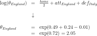
With suitable non-informative priors for the remaining parameters, 4 parallel MCMC chains were run to sample from the underlying probability distributions, and the Gelman-Rubin diagnostic was used to check for convergence to a stationary distribution. With these parameters, we can estimate the probability of any particular score between two teams. For instance, my team England have a mean estimated attack parameter of 0.24, while their first world cup opponents Italy have a mean defence parameter of -0.01. As they will be playing on neutral ground, I halve the home fixed effect and apply it to both sides; this means that number of goals scored by England against Italy is assumed to follow a poisson distribution with rate:

 

Using the probability mass formula for the Poisson distribution, we can now see that the probability of England not scoring is:

As we have assumed that the number of goals scored by each team are independent, the probability of a particular score-line is simply the product of the corresponding goal-scoring probabilities. We can therefore easily predict the probability of any result under the given assumptions. For instance, the probability of Italy also failing to register, calculated in a similar manner as above, is 0.19, and so the probability of no goals in the match is estimated to be 0.12*0.19 = 0.02 – a very low probability. Hopefully the game will be entertaining!

Using this model, then, I simulated the results of the whole tournament 10000 times, sampling each time a set of parameters from the posterior distribution generated by the MCMC algorithm. According to these simulations, the top 6 teams ranked by the proportion of simulations won are displayed in the table below:

Team	Proportion of simulations won
Brazil	39.5%
Netherlands	7.2%
Argentina	6.8%
Germany	6.7%
Spain	5.0%
England	4.8%

In common with more considered simulations conducted elsewhere, Brazil are predicted as the most likely to lift the cup on the 13^th July. In this case, Brazil’s triumph is largely due to the estimated effect of the home advantage, which is considerable. We should also note that the model certainly rests on some questionable assumptions. In particular, the old adage that ‘you are most vulnerable when you’ve just scored’, although debatable, certainly draws attention to the fact that scoring and conceding goals are not independent processes: work by Dixon and Robinson seems to confirm these worries, as they find that the rate of goal scoring for both sides depends upon the score at the time. Furthermore, predicted results appeared to be higher-scoring than one might expect – perhaps because of the nature of the data used to fit the model, where seeding systems disproportionately matched strong teams against weak teams. If this exercise was being carried out ‘for real’, greater effort could be expended in testing different approaches, for instance by holding back observations to test predictive efficacy.

So what does this have to do with demography? Not a lot, you may well think. However, I believe that a couple of points are worth drawing attention to. Over the past couple of decades, there has been an increasing clamour for conducting probabilistic forecasts in demography, in part because it allows a coherent approach to policy making. The above prediction model helps elucidate why, as it assigns a probability to any particular set of results, which enables, for instance, a decision to be made over a sensible set of wagers to be placed on the outcomes of matches or the progression of various teams (although I certainly wouldn’t recommend it!). A similar logic is suggested for making decisions over policy.

Secondly, a Bayesian framework allows the inclusion of subjective or objective priors, as I have done in a rather haphazard way with the information on team rankings. Demographic forecasts can be and have been augmented by including prior information in the form of the elicited opinions of demographic experts. In this model, including only flat priors and not exploiting the extra information we have about team quality meant that the performance of teams from weaker confederation – who played on average easier matches – appeared to be over-estimated. This effect was much less pronounced once priors based on rankings were introduced.

Jason would greatly appreciate comments and any criticism of the above, rather ad-hoc, approach!

Tags: Forecasting, World Cup